On this page
General information only — not financial, investment, legal, or tax advice. Verify all data independently and seek professional advice before making investment decisions. Full disclaimer.
A specialty retail lease signed in the wrong catchment can burn cash for a decade — no early break, no renegotiation, no exit until the term runs out. Regional averages and national vacancy rates won't prevent that — retail supply and demand is hyper-local, and the only analysis that matters is that which is tailored to your specific site within its realistic trade area, with every competing retailer accounted for.
Essential spend categories, constrained new supply, and a population that is both growing and changing in composition underpin retail demand across Australia. The question is not whether people need retail; it is whether a specific site can capture enough of its catchment to make the lease economics work.
Why one metric is never enough: {EXAMPLE_HIGH_NAME} and {EXAMPLE_LOW_NAME} are two SA4 regions in the same metro. One has {EXAMPLE_LOW_SUPERMARKET_POP_PER} people per supermarket; the other has {EXAMPLE_HIGH_SUPERMARKET_POP_PER}. On the surface, the lower ratio signals oversupply. But one of these regions has {EXAMPLE_HIGH_WORKERS_PER_100} workers for every 100 residents — a daily demand pool far larger than the resident count suggests. Grasping the full supply picture always requires effective-population analysis at the site level. A site inside the "well-supplied" region can turn out genuinely undersupplied once its position relative to competitors and population blocks are accounted for, while factors such as increased daytime activity can tip the scales significantly. Worked example →
AreaSearch tracks {RETAIL_TOTAL_BRAND_COUNT} retail brands across {RETAIL_LOCATION_COUNT} Australian locations — every Coles, Woolworths, Aldi, McDonald's, KFC, Bunnings, Anytime Fitness and several hundred others, classified into {RETAIL_CATEGORY_COUNT} categories. Supermarket pop-per-store across metro SA4 regions ranges from {PPS_SPREAD_LOW} to {PPS_SPREAD_HIGH} — a {PPS_SPREAD_RATIO} spread. The five regions with the highest ratio:
- {TOP_PPS_AREA_1} — {TOP_PPS_VALUE_1} people per supermarket
- {TOP_PPS_AREA_2} — {TOP_PPS_VALUE_2}
- {TOP_PPS_AREA_3} — {TOP_PPS_VALUE_3}
- {TOP_PPS_AREA_4} — {TOP_PPS_VALUE_4}
- {TOP_PPS_AREA_5} — {TOP_PPS_VALUE_5}
01The opportunity right now
What makes retail property a compelling asset class — from both sides of the lease
Retail is the only property class where the operator's revenue is a direct function of consumer spending in the catchment — not government funding, not a regulated fee schedule, not a supply chain contract. The landlord earns contracted, CPI-linked income; the operator earns a margin on foot traffic. The economics are different, but they share the same denominator: catchment depth. A growing catchment lifts operator turnover, which secures the lease, which lifts the asset value. And with dozens of retail sub-sectors competing for space at every scale, the opportunity often sits in catchments where the gap between spending capacity and existing supply has not yet been identified.
| Landlord | Operator |
|---|---|
| Long, contracted income — 5–20yr leases with built-in CPI escalation. Few asset classes offer this certainty. | Physical retail is sticky — haircuts, coffee, groceries, gyms. Many categories resist online substitution. |
| Inflation hedge — CPI-linked rent reviews mean income grows with the economy. | Predictable cost base — fixed rent with known escalation means plannable margins year on year. |
| Yield premium — retail cap rates sit above other commercial asset classes for comparable lease quality. | Scalable, repeatable formats — a proven model can be rolled out across new markets. The unit economics travel. |
| Population growth drives demand for space — more people in the catchment means deeper tenant demand and stronger rents. | Population growth expands the customer base — more people in the catchment means more revenue through the door. |
| Non-discretionary tenants are resilient — essential retail holds through economic cycles, protecting income. | Essential spend is recession-proof — people do not stop buying groceries in a downturn. |
| Format diversity — dozens of sub-sectors competing for sites, across every price and risk tier. | Format diversity — entry points at every scale and risk level, from convenience to large format. |
Scale of the sector
Australia's retail market spans over {PCA_TOTAL_CENTRES_AUS} managed shopping centres and {ALL_RETAIL_LOCATIONS} individual major brand retail locations across {RETAIL_CATEGORY_COUNT} distinct categories, from full-line supermarkets through pharmacies, QSR, health and beauty, and large-format bulky goods. Household consumption, the spending that fills these stores, is growing at {HHC_TOTAL_YOY} year-on-year.
Australia's structural tailwinds
Australia's population has passed {AUS_POP_LATEST_M}, with net overseas migration adding {AUS_NOM_LATEST} a year, moderating from its post-COVID peak, but still a large and sustained inflow. Each new household needs groceries, pharmacy, healthcare, hospitality, and personal services within reach. That demand translates directly into more potential customers within reach of any given retail site, and unlike most developed economies, Australia's population growth is a structural feature of the market, not a cyclical one.
The online resilience story
Online retail accounts for roughly {ONLINE_RETAIL_SHARE} of total retail spending nationally, a figure that surged during COVID and has kept climbing since, though the pace has eased. Within that, food and grocery sits at just {ONLINE_GROCERY_SHARE} online penetration, reflecting the structural advantages of physical grocery: freshness, immediacy, and basket complexity. Non-food categories run higher at around {ONLINE_NONFOOD_SHARE}, but growth has flattened. The categories that anchor most retail assets — supermarkets, pharmacies, medical services, QSR, gyms, hair and beauty, cafés — are inherently physical. A well-located centre with the right tenant mix is not competing with e-commerce; it is serving the demand that e-commerce cannot reach.
Yield and return context
Retail property offers a yield premium over other commercial classes for comparable lease quality. Prime regional shopping centres currently transact at {CAP_RATE_REGIONAL} capitalisation rates, neighbourhood centres (typically supermarket-anchored) at {CAP_RATE_NEIGHBOURHOOD}, and large-format retail at {CAP_RATE_LARGE_FORMAT}. Shopping centre vacancy is tight: regional centres at {VACANCY_REGIONAL}, sub-regional at {VACANCY_SUB_REGIONAL}, and prime shopping centre space near {VACANCY_PRIME_RETAIL} nationally. CBD high-street retail is a different story — vacancy has been falling, most recently to {VACANCY_CBD_RETAIL}, still elevated relative to enclosed centres but on a compressing trajectory as foot traffic recovers.
The diversity of retail as an asset class
The sector covers a uniquely wide range of formats — standalone convenience pads, neighbourhood, sub-regional and regional shopping centres, strip retail, large-format bulky goods, and single-tenant net-lease investments. Each carries a different risk profile, tenant covenant, lease structure, and capital requirement. A neighbourhood centre anchored by a major supermarket on a 15-year lease is a fundamentally different proposition from a strip of specialty tenants on 3-year terms, or a standalone QSR pad on a highway corridor. This diversity means there is an entry point at every scale and risk appetite, and that the analytical framework for assessing one format does not transfer directly to another.
Cyclical position
The RBA cash rate sits at {CASH_RATE_CURRENT}, above its 10-year average of {CASH_RATE_10YR_AVG}, a headwind for valuations but increasingly priced in. National unemployment holds at {AUS_UNEMP_CURRENT}, consistent with full employment. Household consumption has been growing at {HHC_TOTAL_YOY} year-on-year, with cafés and restaurants running stronger at {HHC_CAFES_YOY}. Non-residential building approvals — the forward indicator for new retail supply — have returned to near their historical average after several years of undersupply, meaning new stock is arriving but not flooding the market. Growing population, steady employment, and rising consumer spending are structural tailwinds, but elevated interest rates and sticky inflation add uncertainty to the cycle. In that environment, essential retail — supermarkets, pharmacies, medical, QSR — remains the most resilient part of the asset class.
AreaSearch's Economics page tracks these macro drivers in real time — cash rate, unemployment, consumption growth, migration, and building approvals — so you can compare regions side by side when weighing opportunities across different markets.
The question is never whether retail is worth investing in. It is whether a specific site supports the economics on both sides of the lease — and that is a catchment question.
Most supply and demand research in this industry gets this wrong. The standard approach — count population from one geographic source, count competitors from another, divide, and compare to a regional average — produces a number that looks precise but is not. The two geographies do not align at any catchment boundary. The "population per store" ratio that most desktop tools produce is built on a denominator from one dataset and a numerator from another, and the gap between them is exactly where marginal site calls hide. The signals that actually move the decision are more granular, and they require both sides of the ratio to come from the same underlying geography — and that is before you even factor in the impact of working population on daytime demand.
02Using AreaSearch for retail
Two starting points — same tools, different entry point
Whether you are a franchise development team scoping new markets, a leasing manager filling vacancies, an operator assessing a specific lease, an investor evaluating a retail asset, or a landlord testing tenant demand — the toolkit is the same. The tools you choose depend on where you are starting from:
I am searching for opportunities
You want to find under-served catchments. You do not have a specific address yet. Start broad, then narrow to candidate sites.
- Use the retail heatmap to scan supply-per-capita pressure by category
- Use Retail Benchmarks for state-by-state context and category-level reads
- Use Target Search to filter nationally on your demographic + supply criteria
- Run a custom catchment around candidate sites to confirm
I have a site to evaluate
A specific address has come across your desk. You need to confirm catchment, supply gap, and spend capacity before committing.
- Read the area profile for the suburb — free, no sign-up
- Generate a custom catchment in the shape you will actually trade from
- Review local supply and demand trends, commentary and regional comparisons instantly
- Check the site fit against lease and fit-out reality (Section 04)
For most users, the area profile is the right starting point — it is free, covers any area in Australia, and gives you detailed demographic data in a single click. It is not a retail-specific tool, but it provides a taster of our demand side coverage which is assessed with far more granularity at the catchment level.
Retail Benchmarks — sector context
The Retail Benchmarks dashboard gives you a regional view that a single area profile cannot. State and metro pop-per-store ratios across {RETAIL_CATEGORY_COUNT} retail categories. Co-location matrices. Distance-to-nearest stats. Use it to build a shortlist of regions worth investigating in depth, and to understand where your candidate site sits relative to the broader market.
The retail heatmap — broad scan
The homepage heatmap lets you toggle retail and demographic layers across the country. Store locations, new residential addresses, pop-per-store ratios, daily population inflows, income, and much more. Within seconds you can identify the regions where supply pressure concentrates for a target use case.
Area and suburb profiles — free taster
Open any suburb or SA2 area profile and read the key sections that matter for retail:
- Population — density and growth. Catchment scale and trajectory. A supermarket averages {SUPERMARKET_POP_PER_AUS} people per store nationally; a discount department store, closer to {DDS_POP_PER_AUS}. The profile shows total population, growth since Census, and forecast growth — a preliminary check on whether a catchment might support a use case.
- Age section. Median age signals which tenant types are likely to fit. QSR drive-thru skews heavily toward younger demographics. 24/7 fitness is {FITNESS_AGE_COHORT}. Premium grocery skews older with higher household income.
- Income section. Median household income tells you which tenant types an area will support and at what price point.
- Employment. Resident industry mix shows you the economic profile of the area — a healthcare-and-education skew signals different spending patterns from a finance-or-construction base. The working population ratio then shows how many workers are actually present in the area relative to residents, pointing to inflows and outflows, impacting daytime retail demand.
- Transport. Rail station proximity boosts quick service food & beverage; arterial and dual road access are drive-thru qualifiers. The profile shows commute mode and public transport share — high PT share means foot-traffic-led models are likely to outperform.
- Development. Residential DA trends signal future population growth — and therefore future demand. Non-residential DAs indicate incoming retail, commercial, and services supply.
Target Search — multi-criteria shortlisting
Target Search is reverse-engineered location analysis. You set percentile thresholds across metrics — top 20% for working population inflows, top 30% for household income, top 40% for population per QSR, above median for retail-trade employment share — and the platform returns a ranked list of areas matching all of them, anywhere in Australia. Pro tier.
Custom catchment — the site-specific decision tool
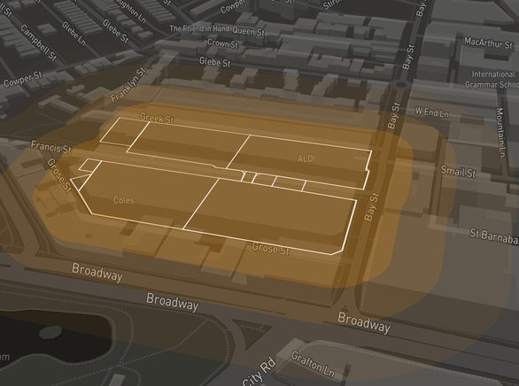
This is the workhorse. Pro tier. Draw a catchment around any address — radius, polygon, or drive-time isochrone — and the platform generates a full site-level report covering demand, supply, competition, demographics, and spending. The Effective Population numbers account for all intersecting competitor catchments, including those outside a drawn boundary, so the competition picture is complete regardless of the shape you draw. The map also carries lot-level planning layers — statutory zoning, development controls such as building height and floor-space ratio, and heritage items.
Every retail report ordered from the website includes a tenancy verification step. The platform's data updates continuously, but before a report is delivered, the tenant register is cross-checked and additional online searches are carried out to catch any missing records, bad geocoding, or cases of retailers not updating their websites. The supply side of the equation is only as good as the tenant count, and this step makes sure nothing is missed.
03The signals that matter
The retail investment metrics that drive value accretion
Total Spending and Category Differentiators
Key Local Employment Industries
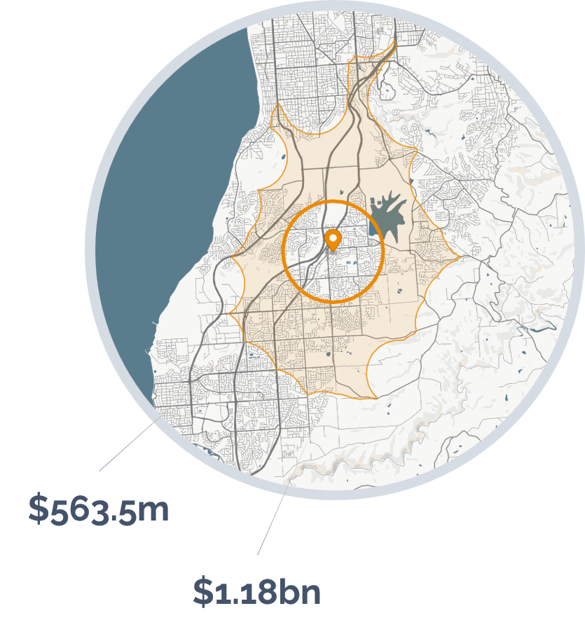
The spending section calculates how much disposable income residents in your catchment actually have, then breaks it down by retail category to show which tenant types the area can support.
Household Income & Costs
| Census median household income | {INCOME_CHAIN_MEDIAN_HHI} |
| + Median-to-mean adjustment | {INCOME_CHAIN_M2M_PCT} |
| + Wage inflation since Census | {INCOME_CHAIN_WAGE_INFL_PCT} |
| = Gross household income | {INCOME_CHAIN_GROSS_HHI} |
| − Net tax burden | {INCOME_CHAIN_TAX_PCT} |
| = After-tax income | {INCOME_CHAIN_AFTER_TAX} |
| − Area-specific housing costs | {INCOME_CHAIN_HOUSING_LATEST} |
| − Savings rate | {INCOME_CHAIN_SAVINGS_RATIO} |
| = Disposable income per household | {INCOME_CHAIN_DISP_POST_SAV} |
| ÷ household size ({INCOME_CHAIN_HH_SIZE}) = per capita | {INCOME_CHAIN_PER_CAPITA} |
Insurance
Restaurants
Spend by category
Per-capita disposable income is allocated across 14 retail categories, with category-level spending shares derived from the ABS Household Expenditure Survey and kept current against five core sources:
- ABS 5204.055011 — Distribution of Household Income, Consumption and Wealth
- ATO Taxation Statistics — Percentile distribution of taxable individuals
- ABS 6401 — CPI by category
- ABS 5206 — Quarterly HFCE, household income and expenditure by state and cohort
- {CENSUS_YEAR} Census — Income and housing costs
The result is a per-capita spending figure for each retail category to compare against state benchmarks, showing where the catchment over and under-indexes before you commit to a position.
Spending projections
The report projects catchment spending forward using 20-year average growth rates for household consumption ({HHC_TOTAL_20YR_CAGR}) and CPI ({CPI_ALL_20YR_CAGR}), blended to a per-capita retail growth rate of {BLENDED_TRADE_CAGR}.
Supply and Demand by Retail Category
Most supply analysis in retail starts and ends with one number: population per store. Count the people, count the stores, divide. The problem is that a simple radius around your site does not all belong to you — some of that population is closer to a competitor, and they will shop there first.
Effective Population (Competition Adjusted Population Capture) corrects for this. AreaSearch divides every catchment into 10 evenly-spaced concentric rings and measures, at each distance, how many people can reach your site relative to how many can reach a competitor. The result is not one number but four:
- Distance to benchmark — the distance at which your effective population meets the regional benchmark.
- Peak Effective Population — the maximum competition-adjusted population across all rings. This is the headline number that underwrites the lease.
- Distance to peak — the ring where peak occurs. Close-in peak = convenience position and likely local dominance. Far-out peak = destination position and often greater competitive risk.
- Market share at peak — your share of the reachable population at the peak distance. Tells you how contested the catchment is at the point that matters most.
Concentric Radial Competition Assessment
The below illustration shows the process using a simple Venn diagram as real world assessments typically encompass dozens of properties, and thousands of population blocks. Effective population is calculated within intersecting segments by dividing the total population count at each increment by the number of intersecting operators.
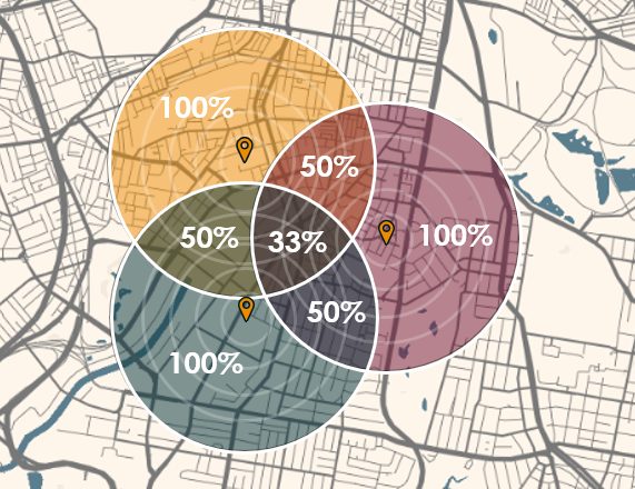
| Total Population | 12,000 | - | 7,000 | - | 14,000 | - | - |
| Segment Population | 6,000 | 1,000 | 2,000 | 1,000 | 8,000 | 2,000 | 3,000 |
| Effective Population | 9,500 | - | 4,000 | - | 10,500 | - | - |
| Market Share % | 79% | - | 57% | - | 75% | - | - |
Where catchments overlap, population is divided by the number of intersecting operators. Effective Population is the competition-adjusted figure that drives sales density.
When charted, this gives insight into changing catchment dynamics across various distances, allowing users to assess primary target markets, changes in market share as competition increases, and ideal distances for promotional activities.
Effective Population by distance ring
Effective Population peaks at 2.1km — beyond that, competition erodes market share. The benchmark line shows the regional average for context.
Effective Population with daily population adjustment
Daily population adjustment adds daytime worker demand to the resident base — material in CBDs and employment precincts.
Daily population within each ring is estimated based on local workforce relative to resident labour force with daytime demand materially exceeding the resident count in built up commercial catchments.
A centre with multiple tenants captures a larger share of population than a single-operator site, but the centre number typically peaks further out — destination retail sees tenants drawing from a broader area in attempts to meet their respective "population per store" benchmarks.
Site vs Centre — Effective Population comparison
Centre EP peaks further out than site EP — the centre must draw from a broader area to support all tenants. The gap between the two lines shows how much tenant diversity adds.
Centre Effective Population with daily adjustment
The full picture for a centre in an employment precinct — competition-adjusted, multi-tenant, and daytime-adjusted demand across all 10 distance rings.
For centres in employment-heavy areas — CBDs, hospital precincts, university corridors — the daily population adjustment layers on top of the centre read.
Choosing the right tenants
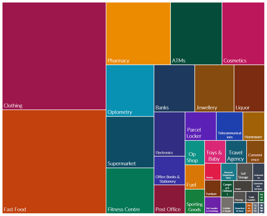
The custom catchment report assesses each of {RETAIL_CATEGORY_COUNT} retail categories individually, measuring two things per category: Effective Population (competition-adjusted demand) and estimated floorspace per capita (existing supply relative to the catchment population). A catchment can be strong for pharmacy, weak for fitness, and a clear opportunity for fast food all at the same time. Understanding the ground realities provides a strong basis for acquisitions, asset repositioning, and sales and leasing campaigns.
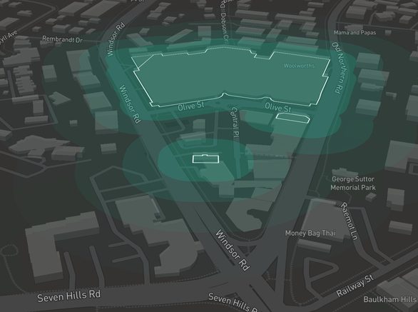
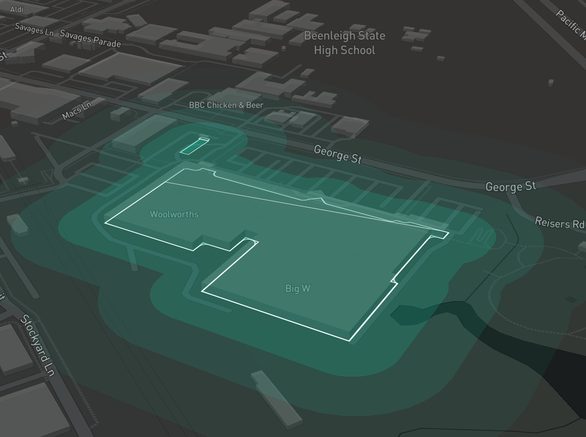
Chains and franchise networks: AreaSearch can assess an entire portfolio — scoring every existing location and shortlisting new ones against cannibalisation buffers, target demographic profiles, and competitor proximity. If you are planning a multi-site rollout or reviewing network performance, get in touch for a portfolio-level engagement.
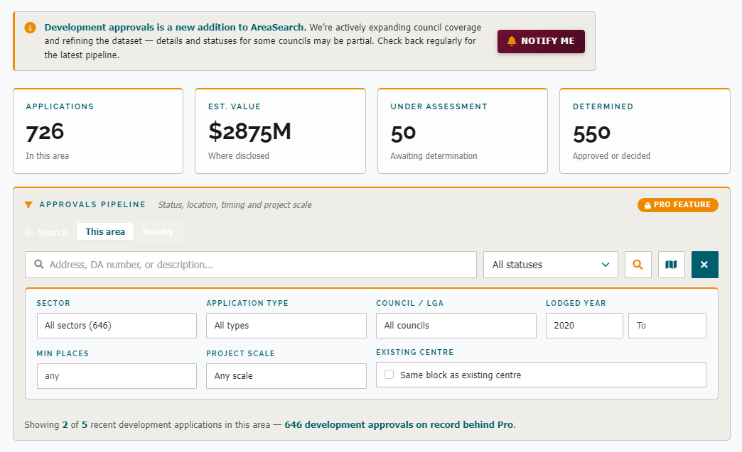
Incoming supply — what is in the DA pipeline
Every supply ratio in this section covers what is already trading. A site that looks under-supplied today can be saturated within {RETAIL_ABSORPTION_TYPICAL} if approved developments are in the pipeline. Council DAs are where the forward supply shows up — approved but not yet built, applications under assessment, and clusters of lodgements that signal other operators have spotted the same opportunity.
AreaSearch's Custom Catchment report scans the DA register within the catchment radius and lists each application — address, status, lodgement date, estimated value, and distance from the site. The report tracks the trailing approval rate and the 12-month count, so you can see whether the pipeline is accelerating or cooling without manually searching council portals.
04The site fit
Lease economics, physical site factors, and fitout due diligence
The occupancy cost ratio (OCR) — and where it breaks
Total occupancy cost (rent + outgoings) as a share of gross sales is the headline lease health number. CBRE's Shopping Centres Australia research puts the national specialty average at {OCR_NATIONAL_AVG} across centre types, well below pre-COVID norms. By tier:
- CBD / super-regional specialty: {OCR_CBD} — still the highest tier
- Sub-regional specialty: {OCR_SUB_REGIONAL}
- Healthy specialty range: {OCR_HEALTHY_RANGE}
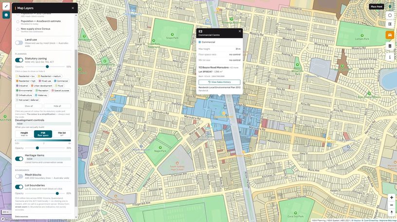
Statutory zoning, development controls and lot boundaries on the map — click any lot for its zoning code and controls.
Lease Portfolio Consultancy frames 20%+ as financial distress for a typical specialty tenant and flags 18%+ as the point where rent realignment should be sought. The ceiling varies by category — a high-margin jeweller can sustain an OCR that would bankrupt a grocer — but as a general rule, specialty tenants trading above 18% of gross sales on occupancy costs are under pressure.
Lease terms — what you are actually signing
- Specialty initial term: {RETAIL_LEASE_TYPICAL_TERM}.
- Anchor initial term: {RETAIL_LEASE_ANCHOR_TERM}.
- Pop-up / short-term: leases under 6 months are exempt from retail lease legislation in most states. Often structured as a licence rather than a lease — fewer protections but faster to set up and exit.
- Subleases: common in centres and CBD retail. The subtenant's rights cannot exceed the head tenant's — if the head lease terminates, the sublease falls with it. Landlord consent is almost always required.
- Outgoings: most new specialty leases are triple-net. Council rates, centre management, insurance, and marketing levies typically add 20–35% on top of headline rent.
- Exclusivity clauses: tenants can negotiate restrictions preventing the landlord from leasing to a direct competitor within the same centre. Common for anchors and strong specialty tenants, but not automatic — the ACCC's exclusive dealing provisions mean overly broad clauses carry competition law risk.
- Demolition clauses, refit obligations, and percentage rent are common in major centres — read these before signing.
- Ground leases: long-term leases (typically 20–50+ years) where the tenant leases the land and builds or owns the improvements. Common with major retail chains on standalone pads — fuel, QSR, hardware, supermarkets. In some cases an investor can secure an Agreement to Lease from a national tenant before exchanging on the site, allowing the acquisition to be funded largely against the tenant covenant — but these deals require significant groundwork: identifying under-valued sites ahead of the market, building relationships with tenant networks, navigating DA risk, and negotiating construction specifications. The investor retains the land and the income stream; the tenant gets a purpose-built site without tying up capital in property ownership.
Regulatory requirements
Every state and territory has its own retail lease legislation. The key protections tenants should know about:
- Mandatory disclosure statement: landlords must provide one at least 7 days before signing (14 days in Victoria and the ACT). If it is missing or materially misleading, the tenant can terminate within 6 months in most states.
- Make-good obligation: most leases require the tenant to strip the fitout and return the premises to base-building condition at lease end. Negotiate scope and caps before signing — this is a common dispute source.
- Accessibility (DDA): the Premises Standards 2010 require retail fitouts to comply with disability access provisions. Both landlord and tenant can be liable for non-compliance.
- Food safety and liquor licensing: food businesses must register with local council and appoint a certified Food Safety Supervisor. Liquor licences are state-issued with lead times of 3–6+ months — factor this into lease commencement timing.
Physical site factors
Beyond the lease numbers, the physical site determines whether a format can actually trade:
- Frontage and signage visibility — street presence and passing traffic exposure
- Customer parking — ratio of spaces to GLA, proximity to entry
- Loading and access — kerbside loading, delivery vehicle access, drive-thru kerb-cut feasibility
- Anchor proximity — co-location with supermarkets or other anchors that generate foot traffic
- Centre environment — if inside a shopping centre, the anchor mix and centre positioning need to match the tenant's target customer
How the calculator works
Select any of the {RETAIL_CATEGORY_COUNT} retail categories AreaSearch tracks to load category-appropriate defaults — effective population (the national benchmark population per store for that category, or an indicative default where AreaSearch's coverage centres on major brands), spend pool, rent, fit-out and construction rates, and margin structure — then adjust to your deal. Effective population is the competition-adjusted population capture for a single store — the output of AreaSearch's Concentric Radials methodology. Use the Tenant or Landlord view to set the deal up from either side. Set the inputs for your store and request your cash flow model — we email you the full model (expected sales, break-even, EBITDA, returns and a month-by-month cash flow over the lease term) built from your settings. Hover any dotted label for a tooltip explaining that input. Use as a screening tool before committing to a full feasibility study.
Retail Returns Calculator
This calculator is a financial modelling tool provided by AreaSearch for indicative analysis only — not investment, tax, or legal advice. Excludes pre-opening capital, working capital during ramp-up, GST, tax, and store-specific factors. Format defaults are illustrative AreaSearch benchmarks — spend pools use narrow trade definitions per category, not total retail spend. Own/Build figures assume a net lease with outgoings fully recovered and interest-only debt where financing is modelled. Seek independent financial advice before committing capital.
05Worked example
{EXAMPLE_HIGH_NAME} vs {EXAMPLE_LOW_NAME} — two SA4 regions in the same metro, with materially different retail supply profiles.
{EXAMPLE_HIGH_NAME} and {EXAMPLE_LOW_NAME} are both SA4 regions in Greater Sydney. Their supermarket pop-per-store ratios — {EXAMPLE_HIGH_SUPERMARKET_POP_PER} and {EXAMPLE_LOW_SUPERMARKET_POP_PER} respectively — suggest different supply levels, and QSR tells a similar story: {EXAMPLE_HIGH_QSR_POP_PER} vs {EXAMPLE_LOW_QSR_POP_PER}. On the surface, the region with the higher ratio looks like the stronger opportunity. The data adds more colour to the story.
| {EXAMPLE_HIGH_NAME} | {EXAMPLE_LOW_NAME} | |
|---|---|---|
| Resident population | {EXAMPLE_HIGH_POP} | {EXAMPLE_LOW_POP} |
| Working population | {EXAMPLE_HIGH_WORKING_POP} | {EXAMPLE_LOW_WORKING_POP} |
| Workers per 100 residents | {EXAMPLE_HIGH_WORKERS_PER_100} | {EXAMPLE_LOW_WORKERS_PER_100} |
| Pop per supermarket | {EXAMPLE_HIGH_SUPERMARKET_POP_PER} | {EXAMPLE_LOW_SUPERMARKET_POP_PER} |
| Pop per QSR | {EXAMPLE_HIGH_QSR_POP_PER} | {EXAMPLE_LOW_QSR_POP_PER} |
| Supermarket count | {EXAMPLE_HIGH_SUPERMARKET_COUNT} | {EXAMPLE_LOW_SUPERMARKET_COUNT} |
| Median household income | {EXAMPLE_HIGH_INCOME} | {EXAMPLE_LOW_INCOME} |
| Population density | {EXAMPLE_HIGH_DENSITY} | {EXAMPLE_LOW_DENSITY} |
| Median age | {EXAMPLE_HIGH_MEDIAN_AGE} | {EXAMPLE_LOW_MEDIAN_AGE} |
| Pop. growth since Census | {EXAMPLE_HIGH_POP_GROWTH} | {EXAMPLE_LOW_POP_GROWTH} |
The pop-per-store ratio uses resident population as its numerator. But {EXAMPLE_HIGH_NAME} has {EXAMPLE_HIGH_WORKERS_PER_100} workers for every 100 residents, a daily demand pool that dwarfs the resident base. {EXAMPLE_LOW_NAME} has {EXAMPLE_LOW_WORKERS_PER_100}. Pop-per-store treats both catchments as if only residents shop there. In one region that is roughly true. In the other, it misses a large part of the demand.
Site-level analysis — where the regional average breaks down
The regional comparison above is useful context, but it is an average across a large area. Retail supply is physically concentrated at specific locations, not spread evenly. A customer's real choice set is the stores within a short drive, regardless of which statistical boundary they fall in. The result: pockets within an "undersupplied" region can be locally saturated, and pockets within a "well-supplied" region can have genuine gaps. Below are two illustrative site catchments that demonstrate exactly this.
Site A — {EXAMPLE_HIGH_NAME}
Illustrative high worker-inflow site · regional pop/supermarket: {EXAMPLE_HIGH_SUPERMARKET_POP_PER}
Low resident base — but massive daily worker inflow
| 800m walk | 5 min drive | |
| Resident population | {SITE_A_RES_POP_NEAR} | {SITE_A_RES_POP_DRIVE} |
| Daily population | {SITE_A_DAILY_POP_NEAR} | {SITE_A_DAILY_POP_DRIVE} |
| Daytime uplift | {SITE_A_UPLIFT_NEAR} | {SITE_A_UPLIFT_DRIVE} |
| SA4 pop/supermarket | {EXAMPLE_HIGH_SUPERMARKET_POP_PER} | |
| Eff. pop / supermarket | {SITE_A_EFF_POP_NEAR} | {SITE_A_EFF_POP_DRIVE} |
{SITE_A_VERDICT}
Site B — {EXAMPLE_LOW_NAME}
Illustrative residential-dominant site · regional pop/supermarket: {EXAMPLE_LOW_SUPERMARKET_POP_PER}
High resident base — but competitor cluster nearby
| 1.5 km | 5 min drive | |
| Resident population | {SITE_B_RES_POP_NEAR} | {SITE_B_RES_POP_DRIVE} |
| Daily population | {SITE_B_DAILY_POP_NEAR} | {SITE_B_DAILY_POP_DRIVE} |
| Daytime uplift | {SITE_B_UPLIFT_NEAR} | {SITE_B_UPLIFT_DRIVE} |
| SA4 pop/supermarket | {EXAMPLE_LOW_SUPERMARKET_POP_PER} | |
| Eff. pop / supermarket | {SITE_B_EFF_POP_NEAR} | {SITE_B_EFF_POP_DRIVE} |
{SITE_B_VERDICT}
The takeaway: the regional pop-per-store ratio pointed one direction; the site-level effective population, accounting for competition and daytime demand, told the opposite story. This is not an anomaly; it is what happens when regional averages smooth over local variation. The regional comparison identifies where to look. The site-level catchment determines whether the opportunity is actually there.
Most underperforming retail sites are not format problems. They are catchment misreads — a daytime-vs-resident error, a competitor cluster hidden inside an assumed trade area, or a household-income floor the format cannot trade through. Each is knowable before the lease is signed.
"{TESTIMONIAL_MINTUS_QUOTE}"
— {TESTIMONIAL_MINTUS_ATTRIBUTION}
Sources: ABS Monthly Household Spending Indicator (MHSI) · {CENSUS_YEAR} Census · Property Council of Australia (Shopping Centre Directory) · CBRE, JLL and Colliers Australian retail research · NAB Online Retail Sales Index · NSW Retail Leases Act 1994, QLD Retail Shop Leases Act 1994, SA Retail and Commercial Leases Act 1995 · AreaSearch analysis. Updated {LATEST_REFRESH_DATE}. This article is a preliminary scoping resource. Make your own enquiries and seek independent professional advice before acting on any information here.